“Navigate the workshop directory and download a dataset.”
“Explain what a library is and what libraries are used for.”
“Describe what the Python Data Analysis Library (Pandas) is.”
“Load the Python Data Analysis Library (Pandas).”
“Use read_csv to read tabular data into Python.”
“Describe what a DataFrame is in Python.”
“Access and summarize data stored in a DataFrame.”
“Define indexing as it relates to data structures.”
“Perform basic mathematical operations and summary statistics on data in a Pandas DataFrame.”
“Create simple plots.”
Automating data analysis tasks in Python
We can automate the process of performing data manipulations in Python. It’s efficient to spend time building the code to perform these tasks because once it’s built, we can use it over and over on different datasets that use a similar format. This makes our methods easily reproducible. We can also easily share our code with colleagues and they can replicate the same analysis.
We will be using this dataset, which can be downloaded here: surveys.csv … but don’t click to download it in your browser - we are going to use Python !
import urllib.request# You can also get this URL value by right-clicking the `surveys.csv` link above and selecting "Copy Link Address"url ='https://monashdatafluency.github.io/python-workshop-base/modules/data/surveys.csv'# url = 'https://goo.gl/9ZxqBg' # or a shortened version to save typingurllib.request.urlretrieve(url, 'surveys.csv')
('surveys.csv', <http.client.HTTPMessage at 0x7f83bca0b9a0>)
If Jupyter is running locally on your computer, you’ll now have a file surveys.csv in the current working directory. You can check by clicking on File tab on the top left of the notebook to see if the file exists. If you are running Jupyter on a remote server or cloud service (eg Colaboratory or Azure Notebooks), the file will be there instead.
We are studying the species and weight of animals caught in plots in our study area. The dataset is stored as a .csv file: each row holds information for a single animal, and the columns represent:
A library in Python contains a set of tools (called functions) that perform tasks on our data. Importing a library is like getting a piece of lab equipment out of a storage locker and setting it up on the bench for use in a project. Once a library is set up, it can be used or called to perform many tasks.
If you have noticed in the previous code import urllib.request, we are calling a request function from library urllib to download our dataset from web.
Pandas in Python
The dataset we have, is in table format. One of the best options for working with tabular data in Python is to use the Python Data Analysis Library (a.k.a. Pandas). The Pandas library provides data structures, produces high quality plots with matplotlib and integrates nicely with other libraries that use NumPy (which is another Python library) arrays.
First, lets make sure the Pandas and matplotlib packages are installed.
!pip install pandas matplotlib
Requirement already satisfied: pandas in /opt/hostedtoolcache/Python/3.10.14/x64/lib/python3.10/site-packages (2.2.2)
Requirement already satisfied: matplotlib in /opt/hostedtoolcache/Python/3.10.14/x64/lib/python3.10/site-packages (3.9.0)
Requirement already satisfied: numpy>=1.22.4 in /opt/hostedtoolcache/Python/3.10.14/x64/lib/python3.10/site-packages (from pandas) (2.0.0)
Requirement already satisfied: python-dateutil>=2.8.2 in /opt/hostedtoolcache/Python/3.10.14/x64/lib/python3.10/site-packages (from pandas) (2.9.0.post0)
Requirement already satisfied: pytz>=2020.1 in /opt/hostedtoolcache/Python/3.10.14/x64/lib/python3.10/site-packages (from pandas) (2024.1)
Requirement already satisfied: tzdata>=2022.7 in /opt/hostedtoolcache/Python/3.10.14/x64/lib/python3.10/site-packages (from pandas) (2024.1)
Requirement already satisfied: contourpy>=1.0.1 in /opt/hostedtoolcache/Python/3.10.14/x64/lib/python3.10/site-packages (from matplotlib) (1.2.1)
Requirement already satisfied: cycler>=0.10 in /opt/hostedtoolcache/Python/3.10.14/x64/lib/python3.10/site-packages (from matplotlib) (0.12.1)
Requirement already satisfied: fonttools>=4.22.0 in /opt/hostedtoolcache/Python/3.10.14/x64/lib/python3.10/site-packages (from matplotlib) (4.53.0)
Requirement already satisfied: kiwisolver>=1.3.1 in /opt/hostedtoolcache/Python/3.10.14/x64/lib/python3.10/site-packages (from matplotlib) (1.4.5)
Requirement already satisfied: packaging>=20.0 in /opt/hostedtoolcache/Python/3.10.14/x64/lib/python3.10/site-packages (from matplotlib) (24.1)
Requirement already satisfied: pillow>=8 in /opt/hostedtoolcache/Python/3.10.14/x64/lib/python3.10/site-packages (from matplotlib) (10.3.0)
Requirement already satisfied: pyparsing>=2.3.1 in /opt/hostedtoolcache/Python/3.10.14/x64/lib/python3.10/site-packages (from matplotlib) (3.1.2)
Requirement already satisfied: six>=1.5 in /opt/hostedtoolcache/Python/3.10.14/x64/lib/python3.10/site-packages (from python-dateutil>=2.8.2->pandas) (1.16.0)

[notice] A new release of pip is available: 24.1 -> 24.1.1
[notice] To update, run: pip install --upgrade pip
Python doesn’t load all of the libraries available to it by default. We have to add an import statement to our code in order to use library functions. To import a library, we use the syntax import libraryName. If we want to give the library a nickname to shorten the command, we can add as nickNameHere. An example of importing the pandas library using the common nickname pd is below.
import pandas as pd
Each time we call a function that’s in a library, we use the syntax LibraryName.FunctionName. Adding the library name with a . before the function name tells Python where to find the function. In the example above, we have imported Pandas as pd. This means we don’t have to type out pandas each time we call a Pandas function.
Reading CSV Data Using Pandas
We will begin by locating and reading our survey data which are in CSV format. CSV stands for Comma-Separated Values and is a common way store formatted data. Other symbols my also be used, so you might see tab-separated, colon-separated or space separated files. It is quite easy to replace one separator with another, to match your application. The first line in the file often has headers to explain what is in each column. CSV (and other separators) make it easy to share data, and can be imported and exported from many applications, including Microsoft Excel.
We can use Pandas’ read_csv function to pull the file directly into a DataFrame.
So What’s a DataFrame?
A DataFrame is a 2-dimensional data structure that can store data of different types (including characters, integers, floating point values, factors and more) in columns. It is similar to a spreadsheet or an SQL table or the data.frame in R. A DataFrame always has an index (0-based). An index refers to the position of an element in the data structure.
# Note that pd.read_csv is used because we imported pandas as pdpd.read_csv("surveys.csv")
record_id
month
day
year
site_id
species_id
sex
hindfoot_length
weight
0
1
7
16
1977
2
NL
M
32.0
NaN
1
2
7
16
1977
3
NL
M
33.0
NaN
2
3
7
16
1977
2
DM
F
37.0
NaN
3
4
7
16
1977
7
DM
M
36.0
NaN
4
5
7
16
1977
3
DM
M
35.0
NaN
...
...
...
...
...
...
...
...
...
...
35544
35545
12
31
2002
15
AH
NaN
NaN
NaN
35545
35546
12
31
2002
15
AH
NaN
NaN
NaN
35546
35547
12
31
2002
10
RM
F
15.0
14.0
35547
35548
12
31
2002
7
DO
M
36.0
51.0
35548
35549
12
31
2002
5
NaN
NaN
NaN
NaN
35549 rows × 9 columns
The above command outputs a DateFrame object, which Jupyter displays as a table (snipped in the middle since there are many rows).
We can see that there were 33,549 rows parsed. Each row has 9 columns. The first column is the index of the DataFrame. The index is used to identify the position of the data, but it is not an actual column of the DataFrame. It looks like the read_csv function in Pandas read our file properly. However, we haven’t saved any data to memory so we can work with it.We need to assign the DataFrame to a variable. Remember that a variable is a name for a value, such as x, or data. We can create a new object with a variable name by assigning a value to it using =.
Let’s call the imported survey data surveys_df:
surveys_df = pd.read_csv("surveys.csv")
Notice when you assign the imported DataFrame to a variable, Python does not produce any output on the screen. We can view the value of the surveys_df object by typing its name into the cell.
surveys_df
record_id
month
day
year
site_id
species_id
sex
hindfoot_length
weight
0
1
7
16
1977
2
NL
M
32.0
NaN
1
2
7
16
1977
3
NL
M
33.0
NaN
2
3
7
16
1977
2
DM
F
37.0
NaN
3
4
7
16
1977
7
DM
M
36.0
NaN
4
5
7
16
1977
3
DM
M
35.0
NaN
...
...
...
...
...
...
...
...
...
...
35544
35545
12
31
2002
15
AH
NaN
NaN
NaN
35545
35546
12
31
2002
15
AH
NaN
NaN
NaN
35546
35547
12
31
2002
10
RM
F
15.0
14.0
35547
35548
12
31
2002
7
DO
M
36.0
51.0
35548
35549
12
31
2002
5
NaN
NaN
NaN
NaN
35549 rows × 9 columns
which prints contents like above.
You can also select just a few rows, so it is easier to fit on one window, you can see that pandas has neatly formatted the data to fit our screen.
Here, we will be using a function called head.
The head() function displays the first several lines of a file. It is discussed below.
surveys_df.head()
record_id
month
day
year
site_id
species_id
sex
hindfoot_length
weight
0
1
7
16
1977
2
NL
M
32.0
NaN
1
2
7
16
1977
3
NL
M
33.0
NaN
2
3
7
16
1977
2
DM
F
37.0
NaN
3
4
7
16
1977
7
DM
M
36.0
NaN
4
5
7
16
1977
3
DM
M
35.0
NaN
Exploring Our Species Survey Data
Again, we can use the type function to see what kind of thing surveys_df is:
type(surveys_df)
pandas.core.frame.DataFrame
As expected, it’s a DataFrame (or, to use the full name that Python uses to refer to it internally, a pandas.core.frame.DataFrame).
What kind of things does surveys_df contain? DataFrames have an attribute called dtypes that answers this:
surveys_df.dtypes
record_id            int64
month                int64
day                  int64
year                 int64
site_id              int64
species_id          object
sex                 object
hindfoot_length    float64
weight             float64
dtype: object
All the values in a single column have the same type. For example, months have type int64, which is a kind of integer. Cells in the month column cannot have fractional values, but the weight and hindfoot_length columns can, because they have type float64. The object type doesn’t have a very helpful name, but in this case it represents strings (such as ‘M’ and ‘F’ in the case of sex).
Useful Ways to View DataFrame objects in Python
There are many ways to summarize and access the data stored in DataFrames, using attributes and methods provided by the DataFrame object.
To access an attribute, use the DataFrame object name followed by the attribute name df_object.attribute. Using the DataFrame surveys_df and attribute columns, an index of all the column names in the DataFrame can be accessed with surveys_df.columns.
Methods are called in a similar fashion using the syntax df_object.method(). As an example, surveys_df.head() gets the first few rows in the DataFrame surveys_df using the head() method. With a method, we can supply extra information in the parens to control behaviour.
Let’s look at the data using these.
Challenge - DataFrames
Using our DataFrame surveys_df, try out the attributes & methods below to see what they return.
surveys_df.columns
surveys_df.shape Take note of the output of shape - what format does it return the shape of the DataFrame in? HINT: More on tuples, here.
surveys_df.head() Also, what does surveys_df.head(15) do?
surveys_df.tail()
Solution - DataFrames
… try it yourself !
Calculating Statistics From Data
We’ve read our data into Python. Next, let’s perform some quick summary statistics to learn more about the data that we’re working with. We might want to know how many animals were collected in each plot, or how many of each species were caught. We can perform summary stats quickly using groups. But first we need to figure out what we want to group by.
Create a list of unique site ID’s found in the surveys data. Call it site_names. How many unique sites are there in the data? How many unique species are in the data?
What is the difference between len(site_names) and surveys_df['site_id'].nunique()?
We often want to calculate summary statistics grouped by subsets or attributes within fields of our data. For example, we might want to calculate the average weight of all individuals per site.
We can calculate basic statistics for all records in a single column using the syntax below:
surveys_df['weight'].describe()
count    32283.000000
mean        42.672428
std         36.631259
min          4.000000
25%         20.000000
50%         37.000000
75%         48.000000
max        280.000000
Name: weight, dtype: float64
We can also extract one specific metric if we wish:
surveys_df['weight'].min()surveys_df['weight'].max()surveys_df['weight'].mean()surveys_df['weight'].std()# only the last command shows output below - you can try the others above in new cellssurveys_df['weight'].count()
np.int64(32283)
But if we want to summarize by one or more variables, for example sex, we can use Pandas’ .groupby method. Once we’ve created a groupby DataFrame, we can quickly calculate summary statistics by a group of our choice.
# Group data by sexgrouped_data = surveys_df.groupby('sex')
The pandas function describe will return descriptive stats including: mean, median, max, min, std and count for a particular column in the data. Note Pandas’ describe function will only return summary values for columns containing numeric data.
# Summary statistics for all numeric columns by sexgrouped_data.describe()# Provide the mean for each numeric column by sex# As above, only the last command shows output below - you can try the others above in new cellsgrouped_data.mean(numeric_only=True)
record_id
month
day
year
site_id
hindfoot_length
weight
sex
F
18036.412046
6.583047
16.007138
1990.644997
11.440854
28.836780
42.170555
M
17754.835601
6.392668
16.184286
1990.480401
11.098282
29.709578
42.995379
The groupby command is powerful in that it allows us to quickly generate summary stats.
Challenge - Summary Data
How many recorded individuals are female F and how many male M
17348 and 15690
14894 and 16476
15303 and 16879
15690 and 17348
What happens when you group by two columns using the following syntax and then grab mean values:
Summarize weight values for each site in your data. HINT: you can use the following syntax to only create summary statistics for one column in your data by_site['weight'].describe()
Solution- Summary Data
## Solution Challenge 1grouped_data.count()
record_id
month
day
year
site_id
species_id
hindfoot_length
weight
sex
F
15690
15690
15690
15690
15690
15690
14894
15303
M
17348
17348
17348
17348
17348
17348
16476
16879
Solution - Challenge 2
The mean value for each combination of site and sex is calculated. Remark that the mean does not make sense for each variable, so you can specify this column-wise: e.g. I want to know the last survey year, median foot-length and mean weight for each site/sex combination:
A Snippet of the Output from part 3 of the challenge looks like:
    site_id
    1     count    1903.000000
          mean       51.822911
          std        38.176670
          min         4.000000
          25%        30.000000
          50%        44.000000
          75%        53.000000
          max       231.000000
         ...
Quickly Creating Summary Counts in Pandas
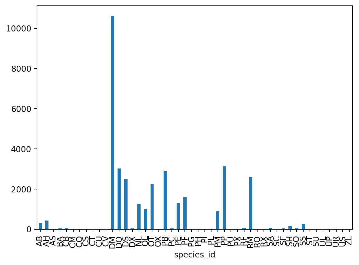
Let’s next count the number of samples for each species. We can do this in a few ways, but we’ll use groupby combined with a count() method.
# Count the number of samples by speciesspecies_counts = surveys_df.groupby('species_id')['record_id'].count()print(species_counts)
species_id
AB      303
AH      437
AS        2
BA       46
CB       50
CM       13
CQ       16
CS        1
CT        1
CU        1
CV        1
DM    10596
DO     3027
DS     2504
DX       40
NL     1252
OL     1006
OT     2249
OX       12
PB     2891
PC       39
PE     1299
PF     1597
PG        8
PH       32
PI        9
PL       36
PM      899
PP     3123
PU        5
PX        6
RF       75
RM     2609
RO        8
RX        2
SA       75
SC        1
SF       43
SH      147
SO       43
SS      248
ST        1
SU        5
UL        4
UP        8
UR       10
US        4
ZL        2
Name: record_id, dtype: int64
Or, we can also count just the rows that have the species “DO”:
If we wanted to, we could perform math on an entire column of our data. For example let’s multiply all weight values by 2. A more practical use of this might be to normalize the data according to a mean, area, or some other value calculated from our data.
# Multiply all weight values by 2 but does not change the original weight datasurveys_df['weight']*2
0          NaN
1          NaN
2          NaN
3          NaN
4          NaN
         ...
35544      NaN
35545      NaN
35546     28.0
35547    102.0
35548      NaN
Name: weight, Length: 35549, dtype: float64
Quick & Easy Plotting Data Using Pandas
We can plot our summary stats using Pandas, too.
## To make sure figures appear inside Jupyter Notebook%matplotlib inline# Create a quick bar chartspecies_counts.plot(kind='bar')
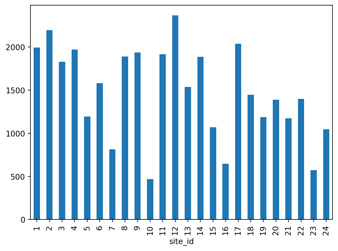
Animals per site plot
We can also look at how many animals were captured in each site.
total_count = surveys_df.groupby('site_id')['record_id'].nunique()# Let's plot that toototal_count.plot(kind='bar')
Extra Plotting Challenge
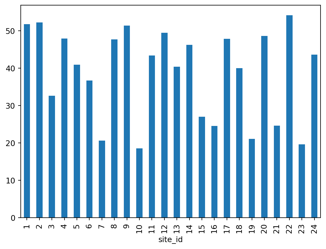
Create a plot of average weight across all species per plot.
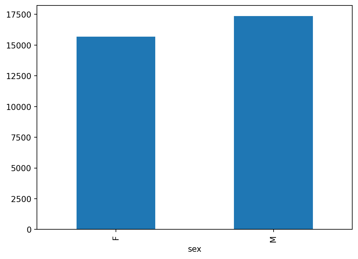
Create a plot of total males versus total females for the entire dataset.
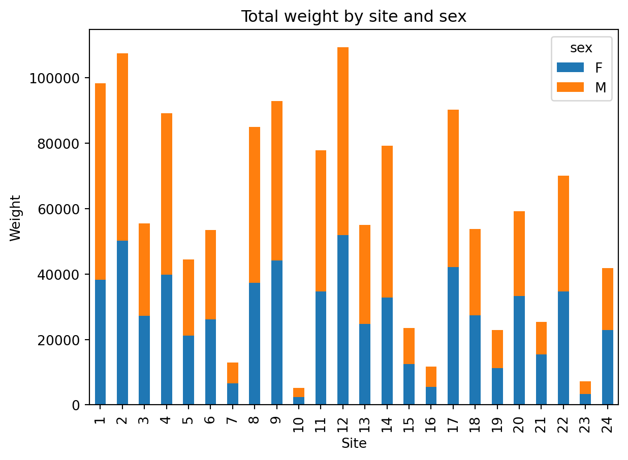
Create a stacked bar plot, with weight on the Y axis, and the stacked variable being sex. The plot should show total weight by sex for each plot. Some tips are below to help you solve this challenge: For more on Pandas plots, visit this link.
# Solution Plotting Challenge 2## Create plot of total males versus total females for the entire dataset.surveys_df.groupby('sex').count()["record_id"].plot(kind='bar')
Solution to Extra Plotting Challenge 3
First we group data by site and by sex, and then calculate a total for each site.